

Technical basics series: A breakdown of Cython basics
Python can already call external C/C++ code from Python. However, Cython greatly simplifies that effort and boosts performance. Learn more about Cytho...
The Team at CallMiner
May 31, 2022


Share
Most of our data is stored in tables called matrices, but there's more to them than just containing data. Their mathematical properties are useful to data science in their own right. Of particular importance to data science is the singular value decomposition or SVD, which provides a ranking of features stored by a matrix.
We'll go over basic matrix math, which is really a bunch of definitions. Then we'll talk about splitting matrices up into useful and informative parts. Finally, I'll go over several applications, including one actually having to do with linguistics.
There are a lot of different kinds of matrices. Most of it is just terminology. We’ll go over some of the greatest hits. We’ll be using the python package numpy to illustrate:
import numpy as npYou may have learned about matrices as solving systems of equations in school at some point. That’s not what I’m going to go over here.
You can start off thinking of a matrix as a grid of numbers. You can characterize them by their shape: “M by N”. M is the number of rows, and N is the number of columns. For example, here’s a 2 x 3 matrix represented in python.
>>> two_by_three=np.array([[6,3,8], [3,4,0]])
>>> two_by_three
array([[6, 3, 8],
       [3, 4, 0]])
If two matrices have the same shape, you can add or subtract them, element by element:
>>>np.add([[6,3,8], [3,4,0]],[[1,1,1],[1,1,1]])
array([[7, 4, 9],
       [4, 5, 1]])
You can multiply a number across a matrix too:
>>>np.multiply([[6,3,8],[3,4,0]],2)
array([[12,  6, 16],
       [ 6,  8,  0]])
If M and N are the same, that’s a square matrix:
>>> square = np.array([[2,3],[5,8]])
>>> square
array([[2, 3],
       [5, 8]])
If you “reflect” the matrix across the diagonal entries, you have made the transpose:
>>> a = np.array([[2,3],[5,8]])
>>> a
array([[2, 3],
       [5, 8]])
>>> np.transpose(a)
array([[2, 5],
       [3, 8]])
If a matrix is equal to its own transpose, it’s called symmetric:
>>> symmetric_matrix = np.array([[9,2,3,4],[2,4,5,3],[3,5,0,7],[4,3,7,1]])
>>> symmetric_matrix
array([[9, 2, 3, 4],
       [2, 4, 5, 3],
       [3, 5, 0, 7],
       [4, 3, 7, 1]])
>>> np.transpose(symmetric_matrix)
array([[9, 2, 3, 4],
       [2, 4, 5, 3],
       [3, 5, 0, 7],
       [4, 3, 7, 1]])
If a matrix only has nonzero entries on the diagonal, it’s called…well, a diagonal matrix:
>>> diagonal_matrix = np.array([[4,0,0],[0,7,0],[0,0,9]])
>>> diagonal_matrix
array([[4, 0, 0],
       [0, 7, 0],
       [0, 0, 9]])
A special diagonal matrix that only has 1s along the diagonal is very important, called the identity matrix:
>>> identity_matrix = np.array([[1,0,0,0],[0,1,0,0],[0,0,1,0],[0,0,0,1]])
>>> identity_matrix
array([[1, 0, 0, 0],
       [0, 1, 0, 0],
       [0, 0, 1, 0],
       [0, 0, 0, 1]])
If you have an M x 1 matrix, that’s a special kind of matrix called a vector. Here’s a 3 x 1 vector:
>>> vector = np.array([[6],[3],[1]])
>>> vector
array([[6],
       [3],
       [1]])
Because it’s got a single column, let’s call it a column vector. As you may guess, there are row vectors too. Here’s a 1 x 4 row vector:
>>> row_vector = np.array([-1,3,8,5])
>>> row_vector
array([-1,  3,  8,  5])
Two matrices can be multiplied together under special conditions: the number of columns of the first matrix must be equal to the number of rows of the second matrix. So I can multiply a 2 x 3 matrix to a 3 x 4 matrix. I can’t multiply a 2 x 3 matrix to a 4 x 3 matrix.
If you can multiply two matrices together, the result will be a matrix with the number of rows of the first and the number of columns of the second. So a 2 x 3 times a 3 x 4 matrix will be a 2 x 4 matrix. (I always imagine the “inner dimension” “canceling out”.
If I multiply a row vector and a column vector. It’s called the inner product or dot product. A row vector has shape 1 x N and a column vector has N x 1, then the result will be a matrix of shape 1 x 1. That’s just a number.*
To compute the dot product, multiply the first element of the row vector by the first element of the column vector, the second element of the row vector times the second element of the column vector, etc. and sum up those products. For example:
>>> np.dot(np.array([-1,3,8,5]), np.array([[1],[2],[3],[4]]))
array([49])
>>> (-1*1)+(3*2)+(8*3)+(5*4)
49
In Python, you can do
>>> import numpy as np
>>> a = np.array([-1, 3, 8, 5])
>>> b = np.array([1, 2, 3, 4])
>>> a @ b  # same as a.dot(b)
49
The length or norm of a vector is the square root of the dot product with itself:
>>> a = np.array([-1,3,8,5])
>>> np.linalg.norm(a)
9.9498743710662
>>> from math import sqrt
>>> sqrt(a @ a) # also np.linalg.norm(a)
9.9498743710662 # sqrt(99)If a vector has a length of 1, it’s called a unit vector. If you’re using Python, don’t confuse this with the len() function! As you can see below, you won’t get the same results.
>>> len(a)
4
>>> np.linalg.norm(a)
9.9498743710662
Even though you don’t need to know how to multiply two matrices together to follow the rest of this, here’s an example. The trick is: take the inner product of row i with column j to get the ij element of the product.
>>> a = np.array([[2,1],[1,2]])
>>> b= np.array([[3,2],[2,3]])
>>> a@b
array([[8, 7],
       [7, 8]])
Order matters in matrix multiplication. Swapping the order is not guaranteed to be the same. In this case, it is the same:
>>> b@a
array([[8, 7],
       [7, 8]])
But in this case, it isn’t:
>>> a = np.array([[2,1],[1,6]])
>>> b= np.array([[3,2],[9,3]])
>>> a@b
array([[15,  7],
       [57, 20]])
>>> b@a
array([[ 8, 15],
       [21, 27]])
Now, let’s say you have some matrix A. If there is another matrix B such that multiplying A and B gives you the identity matrix: “AB= I”. Then B is called the inverse of A and is usually given a special symbol “A-1”
The inverse “undoes” whatever A does. A lot of practical problems in ML, data science, and more would be easily solved if you could calculate the inverse. A classic problem in all these fields looks like “Ax= b”
A and b are known, and you want to compute the unknown vector x. If you knew the inverse of A, then just multiply the inverse on both sides:
A^-1*A*x = A^-1*b
I*x = x = A-1*b
However, as you may expect, calculating the inverse is very expensive as the matrix becomes large. And even if it didn’t take a long time, numerical stability of the algorithm is important. And not all matrices even have an inverse.
However, some special matrices have a very easy way of calculating the inverse:
Q^T*Q = I
OR
Q^T= Q^-1
Your eyes aren’t deceiving you: for this special matrix Q, the inverse is just the transpose. Flip the matrix and you solved your problem! These matrices are called orthogonal.
Now if only there were a way to transform my original matrix into some orthogonal ones…we’ll come back to that in the next section.
The last concept that we need to discuss is the idea of matrix rank. To understand it, take a look at the following matrix. Does anything look odd to you?
>>> weird_matrix = np.array([[1,2,5],[1,2,5],[1,2,5]])
>>> weird_matrix
array([[1, 2, 5],
       [1, 2, 5],
       [1, 2, 5]])
You may have said
Both of these observations are useful. Let’s use the column observation. What this tells us is that the second and third columns are in fact redundant and that there is only one independent column in the matrix. A column is independent if it can’t be written as a combination of the others. We say that the rank of this matrix is the number of independent columns it has: 1, in this case.
Here’s another one:
>>> another_weird_matrix = np.array([[1,3,8],[1,2,6],[0,1,2]])
>>> another_weird_matrix
array([[1, 3, 8],
       [1, 2, 6],
       [0, 1, 2]])
If you stare at this long enough, you can see that the third column is 2 times the first plus 2 times the second. So the third column is redundant, and it turns out the other two can’t be written as combinations of each other. So the rank of this matrix is 2.
Finally,
>>> identity_3= np.array([[1,0,0],[0,1,0],[0,0,1]])
>>> identity_3
array([[1, 0, 0],
       [0, 1, 0],
       [0, 0, 1]])
This matrix has rank 3, or “full rank”.
The singular value decomposition (SVD) is a matrix factorization. Let’s talk about matrix factorizations (or decompositions) first. What are they, and why would anyone want to perform them?
Think about Fourier analysis, where you decompose an audio signal into a sum of sine and cosine waves. This spectral decomposition gives you insight into the sounds you hear.
Likewise, let’s say I have a feature matrix A, with m rows (training examples) and n columns (features). And let’s say that somehow I could factor this matrix into two matrices X and Y, so that A = X*Y.
What are the dimensions of matrices X and Y? Let’s say X has a shape of (m by k), and Y has a shape of (k by n). (Quick check: multiply an (m by k) with a (k by n) and that gives you an (m by n) matrix, good.)
What have we gained from this? Actually, a lot:
Let’s look at a simple factorization of the rank-1 matrix from before:
>>> rank_1_matrix = np.array([[1,2,5],[1,2,5],[1,2,5]])
>>> rank_1_matrix
array([[1, 2, 5],
       [1, 2, 5],
       [1, 2, 5]])
I can “split” this 3 x 3 matrix into a 3 x 1 matrix (column vector) and a 1 x 3 matrix (row vector):
>>> u = np.array([[1],[1],[1]])
>>> u
array([[1],
       [1],
       [1]])
>>> v = np.array([[1],[2],[5]])
>>> v
array([[1],
       [2],
       [5]])
>>> u_times_transpose_v= u @ np.transpose(v)
>>> u_times_transpose_v
array([[1, 2, 5],
       [1, 2, 5],
       [1, 2, 5]])
>>> np.array_equiv(rank_1_matrix, u_times_transpose_v)
True
This product of a column vector and a row vector is called an outer product and always yields an m-by-n matrix. What I just did is “run it in reverse” and decomposed the matrix. It turns out that you can decompose any matrix as a sum of rank-1 matrices. Any rank-1 matrix can be written as a column vector “outer product”-ed with a row vector. This will come in handy later.
The singular value decomposition is the most important theorem in data science.
-Gilbert Strang, 2019
The SVD is useful for conceptual purposes, besides its essential step in algorithms. Many questions in linear algebra can be better understood if we first ask the question, “What if we take the SVD?”
-Trefethen and Bau, 1997
We have finally arrived.
There are many different kinds of matrix factorizations, but none are as general and supreme and awesome as the SVD. It applies to any matrix of any shape unlike most of them.
Let A be an (m by n) matrix. The SVD of A is:
A = USVT
m * n = (m*k) * (k*k) * (k*n)
Here, S is a (k by k) diagonal matrix:
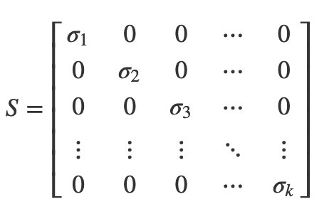
The sigmas along the diagonal are called singular values. (“Singular” here means “really important”.)
The U and V matrices are orthogonal, meaning their inverses are easy to compute; just flip’em!
U-1 = UT
V-1 = VT
I’m not showing you how to calculate one of these by hand because it gets painful as the matrices get bigger. I’d rather show you how to use it and why it’s important. Here’s an example I worked out by hand though!
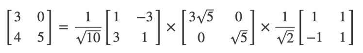
You can play along in Python:
>>> A = np.array( [[3,0],[4,5]] )
>>> U, S, Vt = np.linalg.svd(A)
>>> U
array([[-0.31622777, -0.9486833 ], # 1/sqrt(10) = 0.316
       [-0.9486833 ,  0.31622777]]) # 3/sqrt(10) = 0.949
>>> U @ U.T # is U orthogonal?
array([[1.00000000e+00, 1.14196599e-16],
       [1.14196599e-16, 1.00000000e+00]])
>>> U.T @ U
array([[1.00000000e+00, 1.14196599e-16],
       [1.14196599e-16, 1.00000000e+00]])
>>> S
array([6.70820393, 2.23606798]) # 3*sqrt(5) = 6.71, sqrt(5) = 2.236
>>> Vt
array([[-0.70710678, -0.70710678], # 1/sqrt(2) = 0.707
       [-0.70710678,  0.70710678]])
>>> Vt @ Vt.T # is V orthogonal?
array([[ 1.00000000e+00, -2.23711432e-17],
       [-2.23711432e-17,  1.00000000e+00]])
>>> Vt.T @ Vt
array([[ 1.00000000e+00, -2.23711432e-17],
       [-2.23711432e-17,  1.00000000e+00]])
# multiply them all back together to check that I get what I started with
>>> U @ np.diag(S) @ Vt
array([[3.00000000e+00, 1.33226763e-15], # <--basically 0
       [4.00000000e+00, 5.00000000e+00]])
Besides a minus sign shuffled around, they are the same!
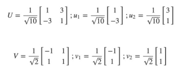
We can think of the columns of U and V as vectors:
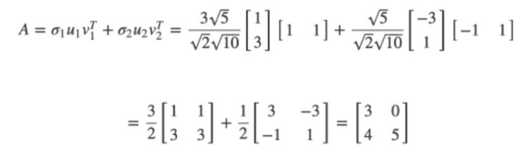
We can rebuild another way: explicitly as the sum of rank-1 matrices:
Great. Now you can compute the SVD in Python. But why does it matter?
You can always write a matrix into a sum of rank-1 pieces. If you arrange the singular values in descending order:
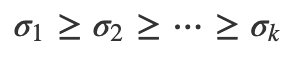
Then you can write the SVD as a sum of terms in order of importance:
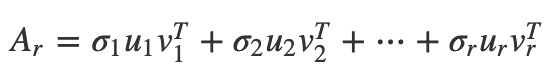
The first part is the closest rank-1 approximation to A. The first two terms are the closest rank-2 approximation to A. The Eckart-Young theorem says that the first r terms are the closest rank-r approximation to A. You can’t do any better! This is the usefulness to data science. If your matrix is too big, a low-rank approximation may be good enough. It may be smaller like any factorization, and using fewer, smarter features may prevent you from overfitting models. This is also why SVDs are often a first step in dimensionality reduction.
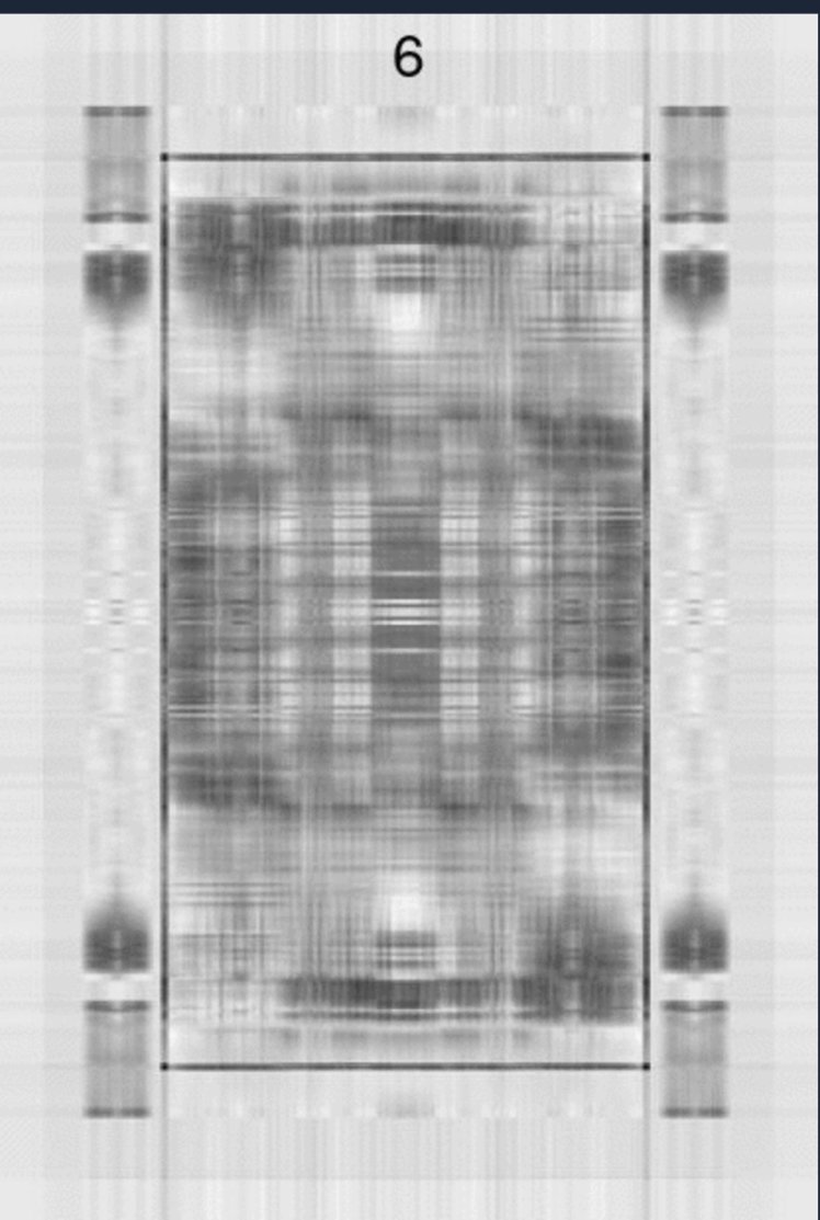
As an illustration of “good enough”, let’s take the SVD of a greyscale image. A greyscale image can be represented by an (m by n) grid of pixels, ranging from 0 - 255. What I’ll show you is successive approximations to the photo, increasing the rank at every iteration. Here’s the original image:

At what rank can we say the image is close enough to a King of Hearts ? At rank 1, it is hard to tell what the image represents.

On the other hand, I can still see errors even at the rank-99 phase.
This image is 612 by 416, so even at rank 100, we’ve omitted 316 “features”. If “good enough” is when you can identify the image, most could guess the image is a King of Hearts by rank-6.
But would this hold true for something more complex or less distinct?
If you took Andrew Ng's machine learning course, you may remember him talking about solving least-squares problems using matrices. The problem: If A is an (m by n) matrix and m is way bigger than n, then there is no exact solution to the matrix equation. But you can find solutions that are close using the following:
A*x = b
Has a least-squares solution given by:
x = (ATA)-1ATb
The important thing here is that inverse. Not all matrices have inverses! Especially when you wish they did. What do you do now? Well, even if the inverse doesn't exist, you can get pretty close with the pseudoinverse (also called the Moore-Penrose matrix). It always exists. It never lets you down. Remember the defining property of an inverse:
AA-1=I
The pseudoinverse promises something a little less committal:
AA+A = A
A+AA+=A+
Pretty close. How do you compute this? Surprise! The first step involves the SVD. If
A=USVT
Then:
A+=VS+UT
The S+ matrix is the same as the diagonal matrix S, except you do the reciprocal of all the entries. Also, if the inverse does exist, then it's the pseudoinverse. Very cool. Here’s a proof of the first property:
AA+A
= (USVT)(VS+UT)(USVT)
= USS+SVT
= USVT
= A
(Maybe) fun fact: Gauss was using equations like this to plot the paths of comets back in the early 1800s. With no computers and definitely no numpy.linalg.pinv, the pseudoinverse in NumPy.
PCA is basically SVD in fancy clothes.
For a while (maybe before autoencoders became important), they were the best way to do dimensionality reduction. Look at this image:
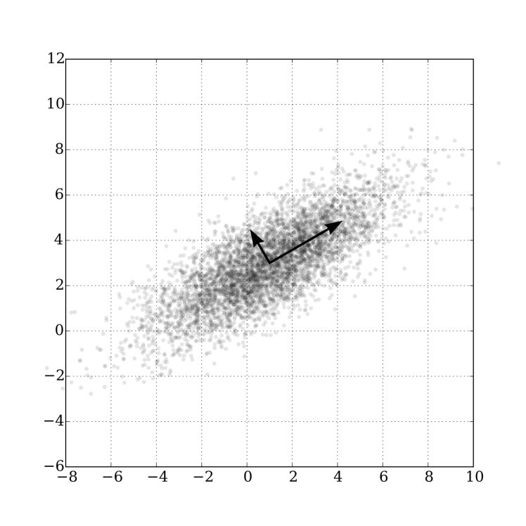
It’s a 2D data set. PCA wants to find the most important directions in the data set. The longer arrow is the first principal component, which means it’s the direction that contains most of the variance in the data set. The second principal component is less important but explains a little more variance. If your data set is high-dimensional, you can keep on going until it’s “good enough”. See what I did there?
Yep. Most PCA implementations are just calling an SVD algorithm. The PCA() in scikit-learn calls randomized_svd directly. For many researchers, PCA and SVD are indistinguishable. Once you understand SVD, you understand PCA (and a lot more).
Let’s use PCA (remember: really the SVD) on some text messages taken from a university lab to see if we can discover topics automatically, particularly spammy ones. Here’s a sample of the data:
tfidf = TfidfVectorizer(tokenizer=casual_tokenize)
tfidf_docs = tfidf.fit_transform(raw_documents = sms.text).toarray()
print("Number of terms from NLTK: ", len(tfidf.vocabulary_))

tfidf_docs = pd.DataFrame(tfidf_docs)
tfidf_docs = tfidf_docs - tfidf_docs.mean() # center the document vectors
print("Shape of TFIDF matrix: ", tfidf_docs.shape)
print("Number of spam messages: ", sms.spam.sum())

Number of terms from NLTK:  9232
Shape of TFIDF matrix:  (4837, 9232)
Number of spam messages:  638
So we have 4837 SMS messages, and 9232 individual terms. Plus, you have way more features (terms, 9232 of them) than you do examples (SMS messages, 4837), and of those messages, only 638 / 4837 = 13% of the data is labeled spam, so it’s imbalanced big time. We’re on our way to overfitting at this rate, because only a few words / features will come out of your model as spammy. A smart spammer will just use synonyms for those spammy words and bypass your filter.
Most people don’t have access to NLP data sets that contain examples of everything people say along with a proper labeling of what they mean. But even if you did, you may run the risk of overfitting. This is how dimensionality reduction comes to the rescue: smaller feature dimensions from words to “topics” can prevent overfitting and make your model more general. This is the essence of latent semantic analysis or LSA, which is PCA applied to NLP, which is the SVD.
Now we can use the SVD directly to do PCA on the data set. Let’s choose 16 components in the SVD (that is, the rank-16 approximation):
# first 10 messages
>>> topics = (topics.T / np.linalg.norm(topics, axis=1)).T # normalize vectors
>>> sim = topics.iloc[:10] @ topics.iloc[:10].T
>>> print(sim.round(1))
       sms0  sms1  sms2!  sms3  sms4  sms5!  sms6  sms7  sms8!  sms9!
sms0    1.0   0.6   -0.1   0.6  -0.0   -0.3  -0.3  -0.1   -0.3   -0.3
sms1    0.6   1.0   -0.2   0.8  -0.2    0.0  -0.2  -0.2   -0.1   -0.1
sms2!  -0.1  -0.2    1.0  -0.2   0.1    0.4   0.0   0.3    0.5    0.4
sms3    0.6   0.8   -0.2   1.0  -0.2   -0.3  -0.1  -0.3   -0.2   -0.1
sms4   -0.0  -0.2    0.1  -0.2   1.0    0.2   0.0   0.1   -0.4   -0.2
sms5!  -0.3   0.0    0.4  -0.3   0.2    1.0  -0.1   0.1    0.3    0.4
sms6   -0.3  -0.2    0.0  -0.1   0.0   -0.1   1.0   0.1   -0.2   -0.2
sms7   -0.1  -0.2    0.3  -0.3   0.1    0.1   0.1   1.0    0.1    0.4
sms8!  -0.3  -0.1    0.5  -0.2  -0.4    0.3  -0.2   0.1    1.0    0.3
sms9!  -0.3  -0.1    0.4  -0.1  -0.2    0.4  -0.2   0.4    0.3    1.0
The spammy messages have a positive similarity score (think: positive correlation) with the other spammy messages here! Also, the non-spammy messages are positively correlated with each other semantically, and crucially, spam is anti-correlated with non-spam.
The spammy messages have a positive similarity score (think: positive correlation) with the other spammy messages here! Also, the non-spammy messages are positively correlated with each other semantically, and crucially, spam is anti-correlated with non-spam.
Unfortunately, this is not true for the whole data set. Two steps forward, one step back?
You may have noticed that I started talking about correlations. There's actually a very interesting connection between correlations and the SVD. In fact, you can use correlation matrices to compute the SVD by hand. If you're bored one day, ask me how.
Combining SVDs with histogram comparison to find important and relevant features!
Footnotes
References
Linear Algebra and Learning From Data (Ch 1)
Natural Language Processing (Ch 14)
Numerical Linear Algebra (Ch 1)
Hands-on Machine Learning with Scikit-Learn and TensorFlow
NLP In Action: Understanding, Analyzing, and Generating Text with Python (Ch 3 & 4)
Introduction to Information Retrieval (Ch 18)
Data Science Design Manual (Ch 8 )
