AWS Machine Learning Blog
Run inference at scale for OpenFold, a PyTorch-based protein folding ML model, using Amazon EKS
This post was co-written with Sachin Kadyan, a leading developer of OpenFold.
In drug discovery, understanding the 3D structure of proteins is key to assessing the ability of a drug to bind to it, directly impacting its efficacy. Predicting the 3D protein form, however, is very complex, challenging, expensive, and time consuming, and can take years when using traditional methods such as X-ray diffraction. Applying machine learning (ML) to predict these structures can significantly accelerate the time to predict protein structures—from years to hours. Several high-profile research teams have released algorithms such as AlphaFold2 (AF2), RoseTTAFold, and others. These algorithms were recognized by Science magazine as the 2021 Breakthrough of the Year.
OpenFold, developed by Columbia University, is an open-source protein structure prediction model implemented with PyTorch. OpenFold is a faithful reproduction of the AlphaFold2 protein structure prediction model, while delivering performance improvements over AlphaFold2. It contains a number of training- and inference-specific optimizations that take advantage of different memory/time trade-offs for different protein lengths based on model training or inference runs. For training, OpenFold supports FlashAttention optimizations that accelerate the multi-sequence alignment (MSA) attention component. FlashAttention optimizations along with JIT compilation accelerate the inference pipeline, delivering twice the performance for shorter protein sequences than AlphaFold2.
For larger protein structures, OpenFold has in-place attention and low-memory attention optimizations, which support predictions of protein structures up to 4,600 residue long, on 40 GB A100 GPU-based Amazon Elastic Compute Cloud (Amazon EC2) p4d instances. Additionally, with memory usage optimization techniques such as CPU offloading, in-place operations, and chunking (splitting input tensors), OpenFold can predict structures for very large proteins that otherwise wouldn’t have been possible with AlphaFold. The alignment pipeline in OpenFold is more efficient than AlphaFold with the HHBlits/JackHMMER toolchain or the much faster MMSeqs2-based MSA generation pipeline.
Columbia University has publicly released the model weights and training data, consisting of 400,000 MSAsand PDB70 template hit files, under a permissive license. Model weights are available via scripts in the GitHub repository, and the MSAs are hosted by the Registry of Open Data on AWS (RODA). Using Python and PyTorch for implementation allows OpenFold to have access to a large array of ML modules and developers, thereby ensuring its continued improvement and optimization.
In this post, we show how you can deploy OpenFold models on Amazon Elastic Kubernetes Service (Amazon EKS) and how to scale the EKS clusters to drastically reduce MSA computation and protein structure inference times. Amazon EKS is a managed container service to run and scale Kubernetes applications on AWS. With Amazon EKS, you can efficiently run distributed training jobs using the latest EC2 instances without needing to install, operate, and maintain your own control plane or nodes. It’s a popular orchestrator for ML and AI workflows, and an increasingly popular container orchestration service in a typical inference architecture for applications like recommendation engines, sentiment analysis, and ad ranking that need to serve a large number of models, with a mix of classical ML and deep learning (DL) models.
We show the performance of this architecture to run alignment computation and inference on the popular open-source Cameo dataset. Running this workload end to end on all 92 proteins available in the Cameo dataset would take a total of 8 hours, which includes downloading the required data, alignment computation, and inference times.
Solution overview
We walk through setting up an EKS cluster using Amazon FSx for Lustre as our distributed file system. We show you how to download the necessary images, model files, container images, and .yaml manifest files. We also show how you can serve the model using FastAPI to predict the 3D protein structure. The MSA step in the protein folding workflow is computationally intensive and can account for a majority of the inference time. In this post, we show how to orchestrate multiple Kubernetes jobs in parallel to use clusters at scale to accelerate the MSA step. Finally, we provide performance comparisons for different compute instances and how you can monitor CPU and GPU utilization.
You can use the reference architecture in this post to test different folding algorithms, test existing pre-trained models on new data, or make performant OpenFold APIs available for broader use in your organization.
Set up the EKS cluster with an FSx for Lustre file system
We use aws-do-eks, an open-source project that provides a large collection of easy-to-use and configurable scripts and tools to enable you to provision EKS clusters and run your inference. To create the cluster using the aws-do-eks repo, follow the steps in the GitHub repository to set up and launch the EKS cluster.If you get an error when creating the cluster, check for these possible reasons:
- If node groups failed to get created because of insufficient capacity, check instance availability in the requested Region and your capacity limits.
- Check that the specified instance type is available or supported in a given AZ.
- EKS cluster creation AWS CloudFormation stacks may not have been properly deleted. You might have to check the active CloudFormation stacks to see if stack deletion has failed.
After the cluster is created, you need the kubectl command line interface (CLI) on the EC2 instance to perform Kubernetes operations. On a Linux instance, run the following command to install the kubectl CLI. Refer to the available commands for any custom requirements.
A typical EKS cluster in AWS looks like the following figure.

We need a scalable shared file system that all compute nodes in the EKS cluster can access. FSx for Lustre is a fully managed, high-performance file system that provides sub-millisecond latencies, up to hundreds of GB/s of throughput, and millions of IOPS. To mount the FSx for Lustre file system to the EKS cluster, refer to Creating File Systems and Copying Data.
You can create the FSx for Lustre file system in the Availability Zone where most of your compute is located to provide the lowest latencies. The file system can be accessed from nodes or pods in any Availability Zone. For simplicity, in this example, we kept the nodes in the same Availability Zone.
Download OpenFold data and model files
Copy the artifacts and protein data banks needed for inference from the Amazon Simple Storage Service (Amazon S3) buckets s3://aws-batch-architecture-for-alphafold-public-artifacts/ and s3://pdbsnapshots/ into the FSx for Lustre file system set up in the previous step. The database consists of AlphaFold parameters, Microbiome analysis data from MGnify, Big Fantastic Database (BFD), Protein Data Bank database, mmCIF files, and PDB SeqRes databases. The scripts to download and unzip the data are available in the download-openfold-data/scripts folder. Use the .yaml file fsx-data-prep-pod.yaml to run a Kubernetes job to download the data. You can launch multiple Kubernetes jobs to accelerate this process, because the file download can be time consuming and take about 4 hours. Complete the following steps to download all data to FSx:
In this example, our shared FSx for Lustre folder is /fsx-shared, which got created after FSx for Lustre volume was mounted on the EKS cluster. When the job is complete, you should see the following folders in the fsx-shared folder.
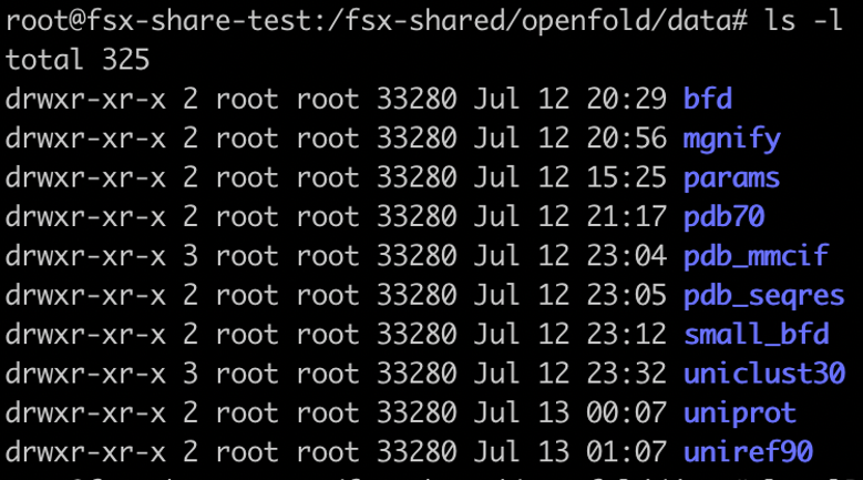
Clone the OpenFold model files and download them into an S3 bucket and from there into an FSx for Lustre file system using the preceding steps. The following screenshot shows the seven files that should be in your FSX file system after you complete the download.

Create an OpenFold Docker file and .yaml manifest file
We have provided an OpenFold Docker file that you can use to build a base container that contains all the necessary dependencies to run OpenFold. To run OpenFold inference with pre-trained OpenFold models, you need to run the following code:
The run_pretrained_openfold.py code provided in the OpenFold GitHub repo is an end-to-end inference code that takes in user inputs and computes alignments if needed using jackhmmer and hhsuite binaries, loads the OpenFold model, and runs inference. It also includes other functionalities, including protein relaxation, model tracing, and multi-model, to name a few. Run the run_pretrained_openfold.py code in a Kubernetes pod using the .yaml file as follows:
Deploy OpenFold models as services and test the solution
To deploy OpenFold model servers as APIs, you need to complete the following steps:
- Update inference_config.properties with information such as OpenFold model name, path to alignment directory, number of models to be deployed per server, model server instance type, number of servers, and server port.
- Build the Docker image with
build.sh. - Push the Docker image with
push.sh. - Deploy the models with
deploy.sh.
If you need to customize the OpenFold APIs, use the fastapi-server.py file, which has all the critical functionality needed to load OpenFold models, compute MSAs, and run inference.
Initialize the model_config, template_featurizer, data_processor, and feature_processor pipelines in fastapi-server.py by calling their respective classes. The precompute_alignment API takes in a protein tag and sequence as optional parameters and generates an alignment if one doesn’t already exist. The alignment_dir variable specifies the location where all the alignments are saved. The precompute_alignment API creates local alignment directories using the tags of each protein sequence. For this reason, make sure tags of each protein are unique. When the API is done running, the bfd_uniclust_hits.a3m, mgnify_hits.a3m, pdb70_hits.hhr, and uniref90_hits.a3m files are created in the local alignment directory.
Call the openfold_predictions inference API, which takes in a protein tag, sequence, and model ID. After the local alignment directory is identified, a processed feature dictionary is created, which gives an input batch. Next, a forward inference call is run with the model to give the output, which must be postprocessed with the prep_output function to yield an unrelaxed protein.
When the fastapi-server.py code is run, it loads multiple OpenFold models on each GPU across multiple instances. To keep track of which model is being loaded on each GPU, we need a global model dictionary that stores the model IDs of each model. You need to specify which checkpoint file you want to use and the number of models to be loaded per GPU, and those models are loaded when the container is run, as shown in the following code:
The inference_config.properties file has inputs that you need to fill, including which checkpoint file to use, instance type for inference, number of model servers, and number of models to be loaded per server. In addition, it includes other inputs corresponding to input arguments in the run_pretrained_openfold.py code, such as number of CPUs, config_preset, and more. If you need to add additional functionality, such as addition protein relaxation, you can add relevant parameters in the inference_config.properties and make relevant changes in the fastapi-server.py code. If you specify models to be run on GPUs and, for example, two model servers with two models to be deployed per server, four Kubernetes applications are deployed (see below).

It’s important to specify the default namespace, otherwise there might be complications accessing FSx for Lustre shared volumes from compute resources in a custom namespace environment.
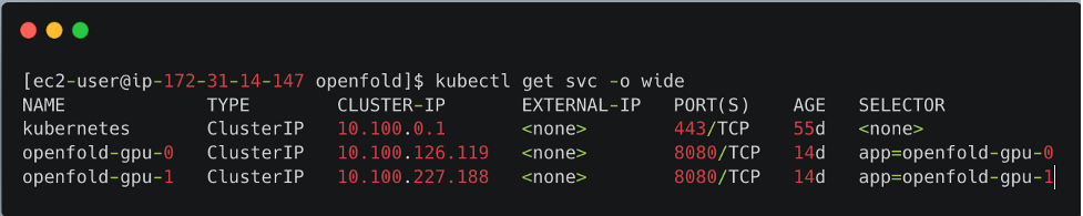
The deploy folder provides the template .yaml manifest file to deploy the OpenFold model as a service and a generate-yaml.sh shell script that creates a .yaml file for each service in a specific folder. For example, if you specify two model servers and p3.2xlarge instance type, openfold-gpu-0.yaml and openfold-gpu-1.yaml files are created in the app-openfold-gpu-p3.2xlarge folder. Then you can deploy the model services as follows:
kubectl apply -f app-openfold-gpu-p3.2xlargeAfter the services are deployed, you can view the deployed services, as shown in the following screenshot.
Run alignment computation
Exposing alignment computation functionality as an API might have some specific use cases, but we need to be able to optimally use the EKS cluster so that alignment computation can be done in a parallel manner. We don’t need expensive GPU-based instances for alignment computation, so we need to add memory- or compute-intensive instances with a large number of CPUs. After we create an EKS cluster, we can create a new node group by running the eks-nodegroup-create.sh script, and we can scale the instances from the auto scaling group on the Amazon EC2 console after we make sure that the instances are in the same Availability Zone as FSx for Lustre. Because alignment computation is more memory intensive, we added r6 instances in the EKS cluster.
The cameo folder contains all the relevant scripts (Docker file; Python code; build, push, and shell scripts; and .yaml manifest file) that showcase how to run compute alignment on a FASTA file of protein sequences. To run alignment computation on your custom FASTA dataset, complete the following steps:
- Save the FASTA file in the FSx folder.
- Create one temporary FASTA file for each protein sequence and save it in the FSx folder.For the Cameo dataset, this is done by running
kubectl apply -f temp-fasta.yamlin thecameo-fastasfolder. - Update the
alignment_dirpath in theprecompute_alignments.pycode, which specifies the destination folder to save the alignments. - Build and push the Docker image to Amazon Elastic Container Registry (Amazon ECR).
- Update the
run-cameo.yamlfile with the instance type and path to the Docker image in Amazon ECR and the number of CPUs if needed. - Update
run-grid.pywith the paths from steps 1 and 2. This code takes in therun-cameo.yamlfile as a template, creates one .yaml file for each alignment computation job, and saves them in thecameo-yamlsfolder. - Finally, submit all the jobs by running
kubectl apply -f cameo-yamls.
The precompute_alignments.py code loads a FASTA file of protein sequences. The run-cameo.yaml file shown in the following code just needs to specify the instance type, shared volume mount specification, and arguments such as number of CPUs for alignment computation:
Depending on the availability of the compute nodes in the cluster, you could submit multiple Kubernetes jobs in parallel. Depending on your needs, you could have one or more dedicated CPU-based instances. After you create a CPU instance type node group, you can easily scale it up or down manually from the Amazon EC2 console. If the need arises for automatic cluster scaling, that could also be possible with the aws-do-eks framework, but would be included in a later iteration of this solution.
Performance tests
We have tested the performance of our architecture on the open-source Cameo dataset. This dataset has a total of 92 proteins of varying lengths. The following plot shows a histogram of the sequence lengths, which has a median sequence length of 236 and four sequences greater than 600.

We generated this plot with the following code:
The alignment computation is memory intensive and not compute intensive, which means that using memory optimized instances will be more cost performant than compute optimized instances. For our tests, we selected the r6i.xlarge instances, which have 4 vCPUs and a 32 GB of memory, and one pod was spun off for one alignment computation job for each protein sequence.
The following table shows the results for the alignment computation jobs. We see that with 92 r6i.xlarge instances, we could complete alignment computation for 92 proteins for under $60. For reference, we compared 1 c6i.12xlarge instance with just one pod that took over 2 days to finish computation.
| Instance Type | Total Memory Available | Total vCPUs Available | Requested Pod Memory | Requested Pod CPUs | Number of Pods | Time Taken | On-Demand Hourly Cost | Total Cost |
| r6i.xlarge | 32 GB | 4 | 16GB | 4 | 92 | 2.5 hours | $0.252/hr | $58 |
| c6i.12xlarge | 96 GB | 48 | Default | 4 | 1 | 49 hours, 43 mins | $2.04/hr | $101 |
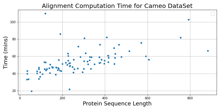
The following plot shows the alignment computation time vs. protein sequence lengths.
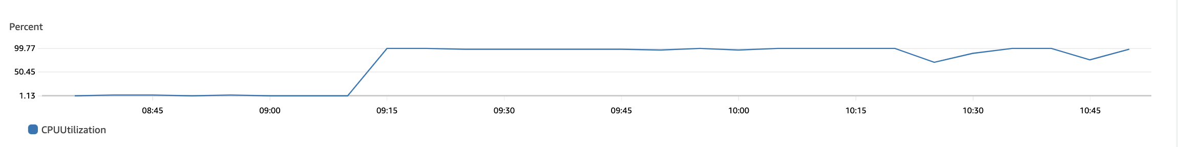
The following plots show max CPU utilization of the 92×4 = 368 vCPUs in the r6i.xlarge auto-scaling group. The bottom plot is just a continuation of the top one. We see that the CPUs were utilized for their maximum capacity and gradually go down to 0 when all jobs finish.

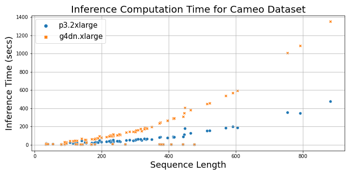
Finally, after the MSAs are computed, we can run the inference by calling the model server APIs. The following table shows the total inference times on the Cameo dataset for p3.2xlarge vs g4dn.xlarge instances. With p3.2xlarge machine, MSA computation over 92 proteins of the Cameo dataset can be done three times faster than g4dn.xlarge machine.
| Instance Type | Number of GPUs | GPU Type | Total vCPUs Available | CPU Memory | GPU Memory | Total Inference Time on Cameo Dataset | On-Demand Hourly Cost | Total Cost |
| p3.2xlarge | 1 | Tesla V100 | 8 | 61 GiB | 16 | 1.36 hours | $3.06/hr | $4 |
| g4dn.xlarge | 1 | Tesla T4 | 4 | 16 GiB | 16 GiB | 3.95 hours | $0.526/hr | $2 |
The following plot shows the total time taken to load the MSA files and perform inference on a p3.2xlarge instance and a g4dn.xlarge instance as a function of protein sequence length. For sequences longer than 200, the inference time with p3.2xlarge instance is three times faster than g4dn.xlarge instance, whereas for shorter sequences, it’s 1–2 times faster.
Clean up
It’s important to spin down resources after model training in order to avoid costs associated with running idle instances. With each script that creates resources, the GitHub repo provides a matching script to delete them. To clean up our setup, we must delete the FSx file system before deleting the cluster, because it’s associated with a subnet in the cluster’s VPC. To delete the FSx file system, run the following command from inside the fsx folder:
Note that this will not only delete the persistent volume, it will also delete the FSx file system, and all the data on the file system will be lost.
When this step is complete, we can delete the cluster by using the following script in the eks folder:
This will delete all the existing pods, remove the cluster, and delete the VPC created in the beginning.
Conclusion
In this post, we showed how to use an EKS cluster to run inference with OpenFold models. We have published the instructions on the AWS EKS Architecture For OpenFold Inference GitHub repo, where you can find step-by-step instructions on how to create an EKS cluster, mount a shared file system to it, download OpenFold data, perform MSA computation, and deploy OpenFold models as APIs. For more information on OpenFold, visit the OpenFold GitHub repo.
About the authors
 Shubha Kumbadakone is a Sr. GTM Specialist for self-managed machine learning with a focus on open-source software and tools. She has more than 17 years of experience in cloud infrastructure and machine learning and is helping customers build their distributed training and inference at scale for their ML models on AWS. She also holds a patent on a caching algorithm for rapid resume from hibernation for mobile systems.
 Ankur Srivastava is a Sr. Solutions Architect in the ML Frameworks Team. He focuses on helping customers with self-managed distributed training and inference at scale on AWS. His experience includes industrial predictive maintenance, digital twins, probabilistic design optimization and has completed his doctoral studies from Mechanical Engineering at Rice University and post-doctoral research from Massachusetts Institute of Technology.
 Sachin Kadyan is a leading developer of OpenFold.