AWS Machine Learning Blog
Monitor embedding drift for LLMs deployed from Amazon SageMaker JumpStart
One of the most useful application patterns for generative AI workloads is Retrieval Augmented Generation (RAG). In the RAG pattern, we find pieces of reference content related to an input prompt by performing similarity searches on embeddings. Embeddings capture the information content in bodies of text, allowing natural language processing (NLP) models to work with language in a numeric form. Embeddings are just vectors of floating point numbers, so we can analyze them to help answer three important questions: Is our reference data changing over time? Are the questions users are asking changing over time? And finally, how well is our reference data covering the questions being asked?
In this post, you’ll learn about some of the considerations for embedding vector analysis and detecting signals of embedding drift. Because embeddings are an important source of data for NLP models in general and generative AI solutions in particular, we need a way to measure whether our embeddings are changing over time (drifting). In this post, you’ll see an example of performing drift detection on embedding vectors using a clustering technique with large language models (LLMS) deployed from Amazon SageMaker JumpStart. You’ll also be able to explore these concepts through two provided examples, including an end-to-end sample application or, optionally, a subset of the application.
Overview of RAG
The RAG pattern lets you retrieve knowledge from external sources, such as PDF documents, wiki articles, or call transcripts, and then use that knowledge to augment the instruction prompt sent to the LLM. This allows the LLM to reference more relevant information when generating a response. For example, if you ask an LLM how to make chocolate chip cookies, it can include information from your own recipe library. In this pattern, the recipe text is converted into embedding vectors using an embedding model, and stored in a vector database. Incoming questions are converted to embeddings, and then the vector database runs a similarity search to find related content. The question and the reference data then go into the prompt for the LLM.
Let’s take a closer look at the embedding vectors that get created and how to perform drift analysis on those vectors.
Analysis on embedding vectors
Embedding vectors are numeric representations of our data so analysis of these vectors can provide insight into our reference data that can later be used to detect potential signals of drift. Embedding vectors represent an item in n-dimensional space, where n is often large. For example, the GPT-J 6B model, used in this post, creates vectors of size 4096. To measure drift, assume that our application captures embedding vectors for both reference data and incoming prompts.
We start by performing dimension reduction using Principal Component Analysis (PCA). PCA tries to reduce the number of dimensions while preserving most of the variance in the data. In this case, we try to find the number of dimensions that preserves 95% of the variance, which should capture anything within two standard deviations.
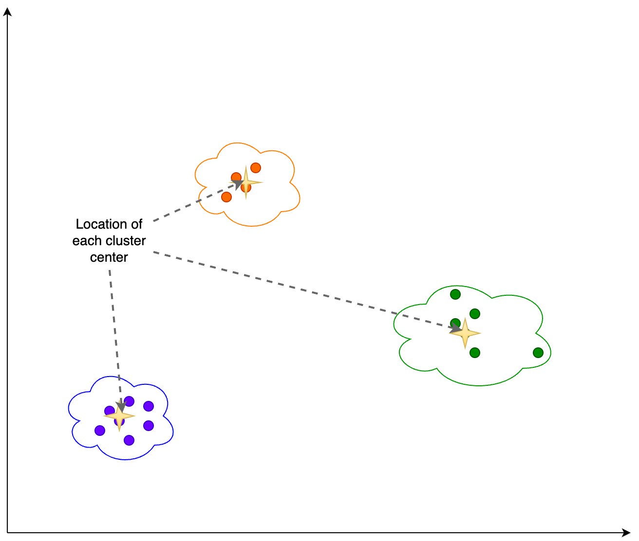
Then we use K-Means to identify a set of cluster centers. K-Means tries to group points together into clusters such that each cluster is relatively compact and the clusters are as distant from each other as possible.
We calculate the following information based on the clustering output shown in the following figure:
- The number of dimensions in PCA that explain 95% of the variance
- The location of each cluster center, or centroid
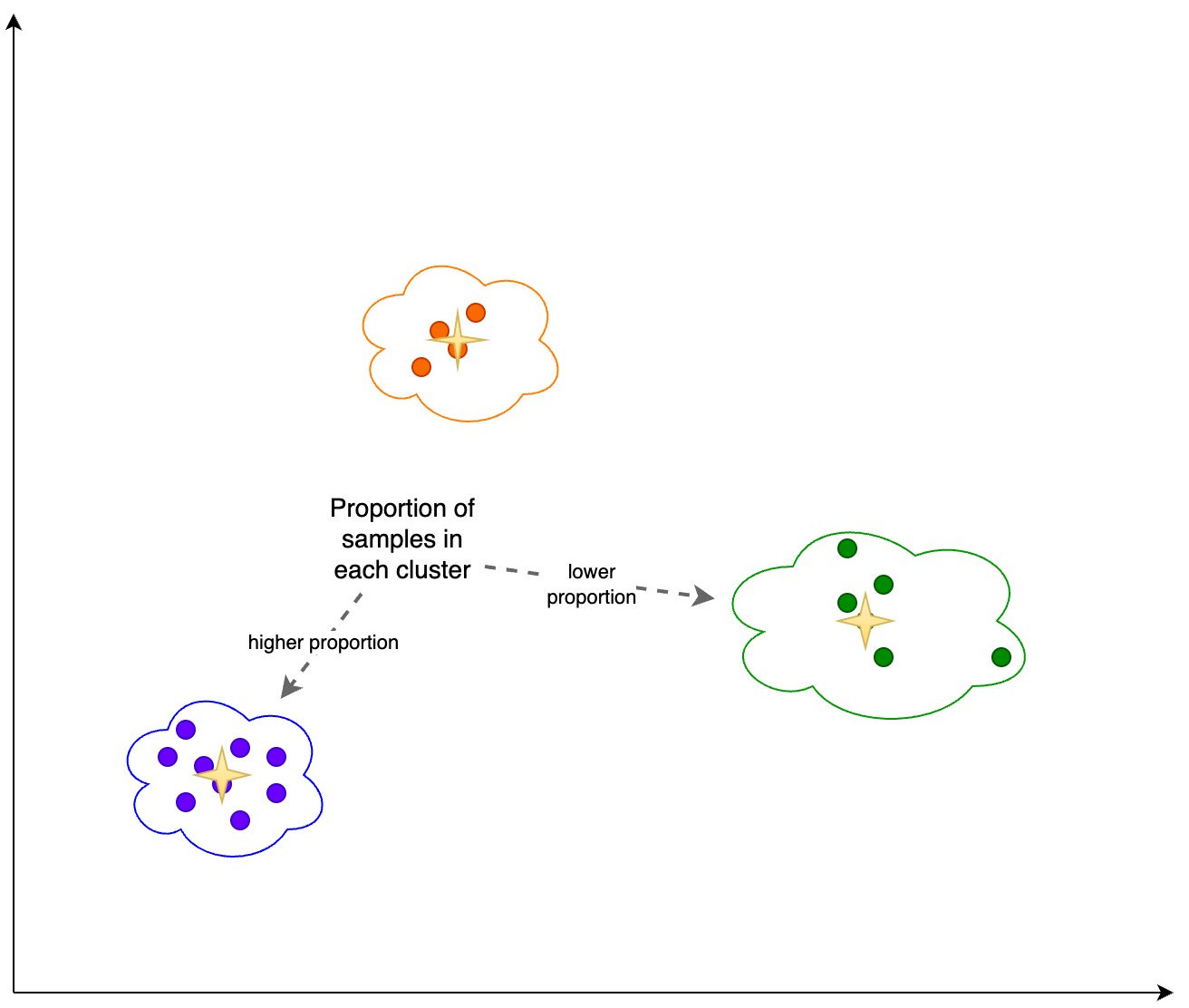
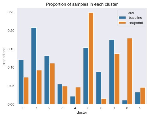
Additionally, we look at the proportion (higher or lower) of samples in each cluster, as shown in the following figure.
Finally, we use this analysis to calculate the following:
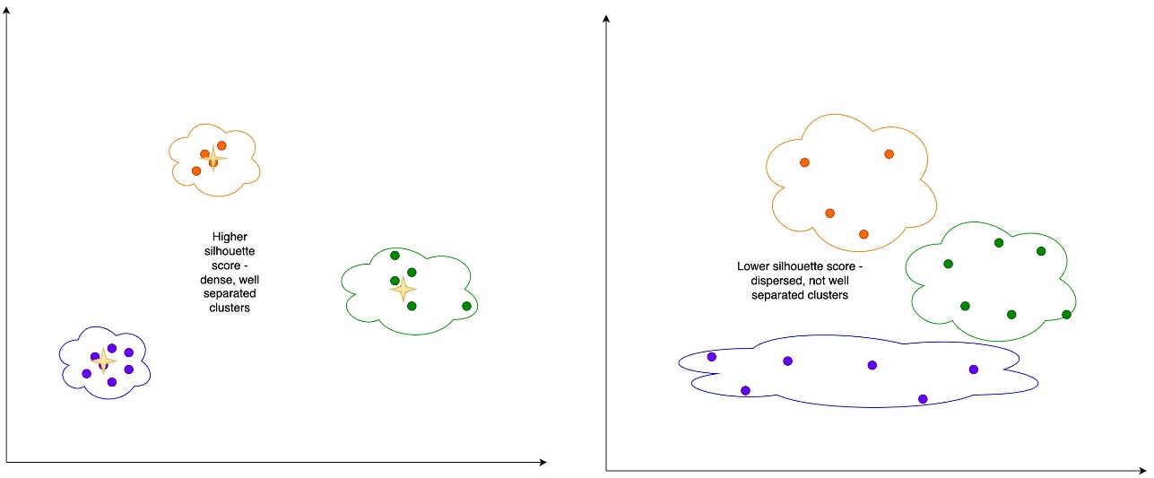
- Inertia – Inertia is the sum of squared distances to cluster centroids, which measures how well the data was clustered using K-Means.
- Silhouette score – The silhouette score is a measure for the validation of the consistency within clusters, and ranges from -1 to 1. A value close to 1 means that the points in a cluster are close to the other points in the same cluster and far from the points of the other clusters. A visual representation of the silhouette score can be seen in the following figure.
We can periodically capture this information for snapshots of the embeddings for both the source reference data and the prompts. Capturing this data allows us to analyze potential signals of embedding drift.
Detecting embedding drift
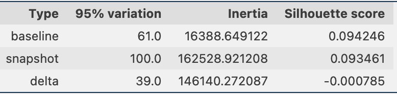
Periodically, we can compare the clustering information through snapshots of the data, which includes the reference data embeddings and the prompt embeddings. First, we can compare the number of dimensions needed to explain 95% of the variation in the embedding data, the inertia, and the silhouette score from the clustering job. As you can see in the following table, compared to a baseline, the latest snapshot of embeddings requires 39 more dimensions to explain the variance, indicating that our data is more dispersed. The inertia has gone up, indicating that the samples are in aggregate farther away from their cluster centers. Additionally, the silhouette score has gone down, indicating that the clusters are not as well defined. For prompt data, that might indicate that the types of questions coming into the system are covering more topics.
Next, in the following figure, we can see how the proportion of samples in each cluster has changed over time. This can show us whether our newer reference data is broadly similar to the previous set, or covers new areas.
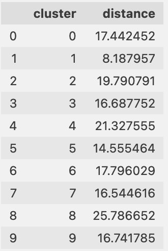
Finally, we can see if the cluster centers are moving, which would show drift in the information in the clusters, as shown in the following table.
Reference data coverage for incoming questions
We can also evaluate how well our reference data aligns to the incoming questions. To do this, we assign each prompt embedding to a reference data cluster. We compute the distance from each prompt to its corresponding center, and look at the mean, median, and standard deviation of those distances. We can store that information and see how it changes over time.
The following figure shows an example of analyzing the distance between the prompt embedding and reference data centers over time.
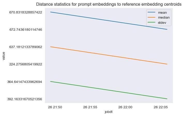
As you can see, the mean, median, and standard deviation distance statistics between prompt embeddings and reference data centers is decreasing between the initial baseline and the latest snapshot. Although the absolute value of the distance is difficult to interpret, we can use the trends to determine if the semantic overlap between reference data and incoming questions is getting better or worse over time.
Sample application
In order to gather the experimental results discussed in the previous section, we built a sample application that implements the RAG pattern using embedding and generation models deployed through SageMaker JumpStart and hosted on Amazon SageMaker real-time endpoints.
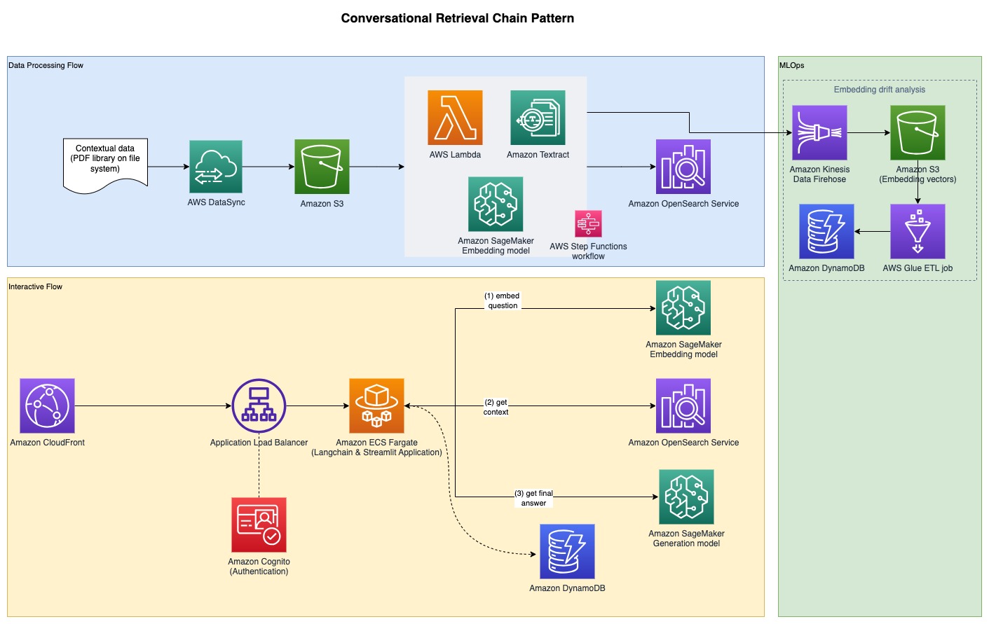
The application has three core components:
- We use an interactive flow, which includes a user interface for capturing prompts, combined with a RAG orchestration layer, using LangChain.
- The data processing flow extracts data from PDF documents and creates embeddings that get stored in Amazon OpenSearch Service. We also use these in the final embedding drift analysis component of the application.
- The embeddings are captured in Amazon Simple Storage Service (Amazon S3) via Amazon Kinesis Data Firehose, and we run a combination of AWS Glue extract, transform, and load (ETL) jobs and Jupyter notebooks to perform the embedding analysis.
The following diagram illustrates the end-to-end architecture.
The full sample code is available on GitHub. The provided code is available in two different patterns:
- Sample full-stack application with a Streamlit frontend – This provides an end-to-end application, including a user interface using Streamlit for capturing prompts, combined with the RAG orchestration layer, using LangChain running on Amazon Elastic Container Service (Amazon ECS) with AWS Fargate
- Backend application – For those that don’t want to deploy the full application stack, you can optionally choose to only deploy the backend AWS Cloud Development Kit (AWS CDK) stack, and then use the Jupyter notebook provided to perform RAG orchestration using LangChain
To create the provided patterns, there are several prerequisites detailed in the following sections, starting with deploying the generative and text embedding models then moving on to the additional prerequisites.
Deploy models through SageMaker JumpStart
Both patterns assume the deployment of an embedding model and generative model. For this, you’ll deploy two models from SageMaker JumpStart. The first model, GPT-J 6B, is used as the embedding model and the second model, Falcon-40b, is used for text generation.
You can deploy each of these models through SageMaker JumpStart from the AWS Management Console, Amazon SageMaker Studio, or programmatically. For more information, refer to How to use JumpStart foundation models. To simplify the deployment, you can use the provided notebook derived from notebooks automatically created by SageMaker JumpStart. This notebook pulls the models from the SageMaker JumpStart ML hub and deploys them to two separate SageMaker real-time endpoints.
The sample notebook also has a cleanup section. Don’t run that section yet, because it will delete the endpoints just deployed. You will complete the cleanup at the end of the walkthrough.
After confirming successful deployment of the endpoints, you’re ready to deploy the full sample application. However, if you’re more interested in exploring only the backend and analysis notebooks, you can optionally deploy only that, which is covered in the next section.
Option 1: Deploy the backend application only
This pattern allows you to deploy the backend solution only and interact with the solution using a Jupyter notebook. Use this pattern if you don’t want to build out the full frontend interface.
Prerequisites
You should have the following prerequisites:
- A SageMaker JumpStart model endpoint deployed – Deploy the models to SageMaker real-time endpoints using SageMaker JumpStart, as previously outlined
- Deployment parameters – Record the following:
- Text model endpoint name – The endpoint name of the text generation model deployed with SageMaker JumpStart
- Embeddings model endpoint name – The endpoint name of the embedding model deployed with SageMaker JumpStart
Deploy the resources using the AWS CDK
Use the deployment parameters noted in the previous section to deploy the AWS CDK stack. For more information about AWS CDK installation, refer to Getting started with the AWS CDK.
Make sure that Docker is installed and running on the workstation that will be used for AWS CDK deployment. Refer to Get Docker for additional guidance.
Alternatively, you can enter the context values in a file called cdk.context.json in the pattern1-rag/cdk directory and run cdk deploy BackendStack --exclusively.
The deployment will print out outputs, some of which will be needed to run the notebook. Before you can start question and answering, embed the reference documents, as shown in the next section.
Embed reference documents
For this RAG approach, reference documents are first embedded with a text embedding model and stored in a vector database. In this solution, an ingestion pipeline has been built that intakes PDF documents.
An Amazon Elastic Compute Cloud (Amazon EC2) instance has been created for the PDF document ingestion and an Amazon Elastic File System (Amazon EFS) file system is mounted on the EC2 instance to save the PDF documents. An AWS DataSync task is run every hour to fetch PDF documents found in the EFS file system path and upload them to an S3 bucket to start the text embedding process. This process embeds the reference documents and saves the embeddings in OpenSearch Service. It also saves an embedding archive to an S3 bucket through Kinesis Data Firehose for later analysis.
To ingest the reference documents, complete the following steps:
- Retrieve the sample EC2 instance ID that was created (see the AWS CDK output
JumpHostId) and connect using Session Manager, a capability of AWS Systems Manager. For instructions, refer to Connect to your Linux instance with AWS Systems Manager Session Manager. - Go to the directory
/mnt/efs/fs1, which is where the EFS file system is mounted, and create a folder calledingest: - Add your reference PDF documents to the
ingestdirectory.
The DataSync task is configured to upload all files found in this directory to Amazon S3 to start the embedding process.
The DataSync task runs on an hourly schedule; you can optionally start the task manually to start the embedding process immediately for the PDF documents you added.
- To start the task, locate the task ID from the AWS CDK output
DataSyncTaskIDand start the task with defaults.
After the embeddings are created, you can start the RAG question and answering through a Jupyter notebook, as shown in the next section.
Question and answering using a Jupyter notebook
Complete the following steps:
- Retrieve the SageMaker notebook instance name from the AWS CDK output
NotebookInstanceNameand connect to JupyterLab from the SageMaker console. - Go to the directory
fmops/full-stack/pattern1-rag/notebooks/. - Open and run the notebook
query-llm.ipynbin the notebook instance to perform question and answering using RAG.
Make sure to use the conda_python3 kernel for the notebook.
This pattern is useful to explore the backend solution without needing to provision additional prerequisites that are required for the full-stack application. The next section covers the implementation of a full-stack application, including both the frontend and backend components, to provide a user interface for interacting with your generative AI application.
Option 2: Deploy the full-stack sample application with a Streamlit frontend
This pattern allows you to deploy the solution with a user frontend interface for question and answering.
Prerequisites
To deploy the sample application, you must have the following prerequisites:
- SageMaker JumpStart model endpoint deployed – Deploy the models to your SageMaker real-time endpoints using SageMaker JumpStart, as outlined in the previous section, using the provided notebooks.
- Amazon Route 53 hosted zone – Create an Amazon Route 53 public hosted zone to use for this solution. You can also use an existing Route 53 public hosted zone, such as
example.com. - AWS Certificate Manager certificate – Provision an AWS Certificate Manager (ACM) TLS certificate for the Route 53 hosted zone domain name and its applicable subdomains, such as
example.comand*.example.comfor all subdomains. For instructions, refer to Requesting a public certificate. This certificate is used to configure HTTPS on Amazon CloudFront and the origin load balancer. - Deployment parameters – Record the following:
- Frontend application custom domain name – A custom domain name used to access the frontend sample application. The domain name provided is used to create a Route 53 DNS record pointing to the frontend CloudFront distribution; for example,
app.example.com. - Load balancer origin custom domain name – A custom domain name used for the CloudFront distribution load balancer origin. The domain name provided is used to create a Route 53 DNS record pointing to the origin load balancer; for example,
app-lb.example.com. - Route 53 hosted zone ID – The Route 53 hosted zone ID to host the custom domain names provided; for example,
ZXXXXXXXXYYYYYYYYY. - Route 53 hosted zone name – The name of the Route 53 hosted zone to host the custom domain names provided; for example,
example.com. - ACM certificate ARN – The ARN of the ACM certificate to be used with the custom domain provided.
- Text model endpoint name – The endpoint name of the text generation model deployed with SageMaker JumpStart.
- Embeddings model endpoint name – The endpoint name of the embedding model deployed with SageMaker JumpStart.
- Frontend application custom domain name – A custom domain name used to access the frontend sample application. The domain name provided is used to create a Route 53 DNS record pointing to the frontend CloudFront distribution; for example,
Deploy the resources using the AWS CDK
Use the deployment parameters you noted in the prerequisites to deploy the AWS CDK stack. For more information, refer to Getting started with the AWS CDK.
Make sure Docker is installed and running on the workstation that will be used for the AWS CDK deployment.
In the preceding code, -c represents a context value, in the form of the required prerequisites, provided on input. Alternatively, you can enter the context values in a file called cdk.context.json in the pattern1-rag/cdk directory and run cdk deploy --all.
Note that we specify the Region in the file bin/cdk.ts. Configuring ALB access logs requires a specified Region. You can change this Region before deployment.
The deployment will print out the URL to access the Streamlit application. Before you can start question and answering, you need to embed the reference documents, as shown in the next section.
Embed the reference documents
For a RAG approach, reference documents are first embedded with a text embedding model and stored in a vector database. In this solution, an ingestion pipeline has been built that intakes PDF documents.
As we discussed in the first deployment option, an example EC2 instance has been created for the PDF document ingestion and an EFS file system is mounted on the EC2 instance to save the PDF documents. A DataSync task is run every hour to fetch PDF documents found in the EFS file system path and upload them to an S3 bucket to start the text embedding process. This process embeds the reference documents and saves the embeddings in OpenSearch Service. It also saves an embedding archive to an S3 bucket through Kinesis Data Firehose for later analysis.
To ingest the reference documents, complete the following steps:
- Retrieve the sample EC2 instance ID that was created (see the AWS CDK output
JumpHostId) and connect using Session Manager. - Go to the directory
/mnt/efs/fs1, which is where the EFS file system is mounted, and create a folder calledingest: - Add your reference PDF documents to the
ingestdirectory.
The DataSync task is configured to upload all files found in this directory to Amazon S3 to start the embedding process.
The DataSync task runs on an hourly schedule. You can optionally start the task manually to start the embedding process immediately for the PDF documents you added.
- To start the task, locate the task ID from the AWS CDK output
DataSyncTaskIDand start the task with defaults.
Question and answering
After the reference documents have been embedded, you can start the RAG question and answering by visiting the URL to access the Streamlit application. An Amazon Cognito authentication layer is used, so it requires creating a user account in the Amazon Cognito user pool deployed via the AWS CDK (see the AWS CDK output for the user pool name) for first-time access to the application. For instructions on creating an Amazon Cognito user, refer to Creating a new user in the AWS Management Console.
Embed drift analysis
In this section, we show you how to perform drift analysis by first creating a baseline of the reference data embeddings and prompt embeddings, and then creating a snapshot of the embeddings over time. This allows you to compare the baseline embeddings to the snapshot embeddings.
Create an embedding baseline for the reference data and prompt
To create an embedding baseline of the reference data, open the AWS Glue console and select the ETL job embedding-drift-analysis. Set the parameters for the ETL job as follows and run the job:
- Set
--job_typetoBASELINE. - Set
--out_tableto the Amazon DynamoDB table for reference embedding data. (See the AWS CDK outputDriftTableReferencefor the table name.) - Set
--centroid_tableto the DynamoDB table for reference centroid data. (See the AWS CDK outputCentroidTableReferencefor the table name.) - Set
--data_pathto the S3 bucket with the prefix; for example,s3://<REPLACE_WITH_BUCKET_NAME>/embeddingarchive/. (See the AWS CDK outputBucketNamefor the bucket name.)
Similarly, using the ETL job embedding-drift-analysis, create an embedding baseline of the prompts. Set the parameters for the ETL job as follows and run the job:
- Set
--job_typetoBASELINE - Set
--out_tableto the DynamoDB table for prompt embedding data. (See the AWS CDK outputDriftTablePromptsNamefor the table name.) - Set
--centroid_tableto the DynamoDB table for prompt centroid data. (See the AWS CDK outputCentroidTablePromptsfor the table name.) - Set
--data_pathto the S3 bucket with the prefix; for example,s3://<REPLACE_WITH_BUCKET_NAME>/promptarchive/. (See the AWS CDK outputBucketNamefor the bucket name.)
Create an embedding snapshot for the reference data and prompt
After you ingest additional information into OpenSearch Service, run the ETL job embedding-drift-analysis again to snapshot the reference data embeddings. The parameters will be the same as the ETL job that you ran to create the embedding baseline of the reference data as shown in the previous section, with the exception of setting the --job_type parameter to SNAPSHOT.
Similarly, to snapshot the prompt embeddings, run the ETL job embedding-drift-analysis again. The parameters will be the same as the ETL job that you ran to create the embedding baseline for the prompts as shown in the previous section, with the exception of setting the --job_type parameter to SNAPSHOT.
Compare the baseline to the snapshot
To compare the embedding baseline and snapshot for reference data and prompts, use the provided notebook pattern1-rag/notebooks/drift-analysis.ipynb.
To look at embedding comparison for reference data or prompts, change the DynamoDB table name variables (tbl and c_tbl) in the notebook to the appropriate DynamoDB table for each run of the notebook.
The notebook variable tbl should be changed to the appropriate drift table name. The following is an example of where to configure the variable in the notebook.
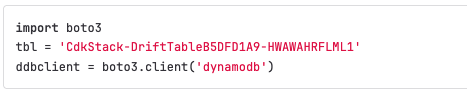
The table names can be retrieved as follows:
- For the reference embedding data, retrieve the drift table name from the AWS CDK output
DriftTableReference - For the prompt embedding data, retrieve the drift table name from the AWS CDK output
DriftTablePromptsName
In addition, the notebook variable c_tbl should be changed to the appropriate centroid table name. The following is an example of where to configure the variable in the notebook.
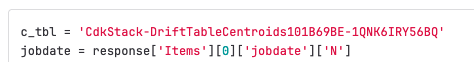
The table names can be retrieved as follows:
- For the reference embedding data, retrieve the centroid table name from the AWS CDK output
CentroidTableReference - For the prompt embedding data, retrieve the centroid table name from the AWS CDK output
CentroidTablePrompts
Analyze the prompt distance from the reference data
First, run the AWS Glue job embedding-distance-analysis. This job will find out which cluster, from the K-Means evaluation of the reference data embeddings, that each prompt belongs to. It then calculates the mean, median, and standard deviation of the distance from each prompt to the center of the corresponding cluster.
You can run the notebook pattern1-rag/notebooks/distance-analysis.ipynb to see the trends in the distance metrics over time. This will give you a sense of the overall trend in the distribution of the prompt embedding distances.
The notebook pattern1-rag/notebooks/prompt-distance-outliers.ipynb is an AWS Glue notebook that looks for outliers, which can help you identify whether you’re getting more prompts that are not related to the reference data.
Monitor similarity scores
All similarity scores from OpenSearch Service are logged in Amazon CloudWatch under the rag namespace. The dashboard RAG_Scores shows the average score and the total number of scores ingested.
Clean up
To avoid incurring future charges, delete all the resources that you created.
Delete the deployed SageMaker models
Reference the cleanup up section of the provided example notebook to delete the deployed SageMaker JumpStart models, or you can delete the models on the SageMaker console.
Delete the AWS CDK resources
If you entered your parameters in a cdk.context.json file, clean up as follows:
If you entered your parameters on the command line and only deployed the backend application (the backend AWS CDK stack), clean up as follows:
If you entered your parameters on the command line and deployed the full solution (the frontend and backend AWS CDK stacks), clean up as follows:
Conclusion
In this post, we provided a working example of an application that captures embedding vectors for both reference data and prompts in the RAG pattern for generative AI. We showed how to perform clustering analysis to determine whether reference or prompt data is drifting over time, and how well the reference data covers the types of questions users are asking. If you detect drift, it can provide a signal that the environment has changed and your model is getting new inputs that it may not be optimized to handle. This allows for proactive evaluation of the current model against changing inputs.
About the Authors
 Abdullahi Olaoye is a Senior Solutions Architect at Amazon Web Services (AWS). Abdullahi holds a MSC in Computer Networking from Wichita State University and is a published author that has held roles across various technology domains such as DevOps, infrastructure modernization and AI. He is currently focused on Generative AI and plays a key role in assisting enterprises to architect and build cutting-edge solutions powered by Generative AI. Beyond the realm of technology, he finds joy in the art of exploration. When not crafting AI solutions, he enjoys traveling with his family to explore new places.
 Randy DeFauw is a Senior Principal Solutions Architect at AWS. He holds an MSEE from the University of Michigan, where he worked on computer vision for autonomous vehicles. He also holds an MBA from Colorado State University. Randy has held a variety of positions in the technology space, ranging from software engineering to product management. In entered the Big Data space in 2013 and continues to explore that area. He is actively working on projects in the ML space and has presented at numerous conferences including Strata and GlueCon.
 Shelbee Eigenbrode is a Principal AI and Machine Learning Specialist Solutions Architect at Amazon Web Services (AWS). She has been in technology for 24 years spanning multiple industries, technologies, and roles. She is currently focusing on combining her DevOps and ML background into the domain of MLOps to help customers deliver and manage ML workloads at scale. With over 35 patents granted across various technology domains, she has a passion for continuous innovation and using data to drive business outcomes. Shelbee is a co-creator and instructor of the Practical Data Science specialization on Coursera. She is also the Co-Director of Women In Big Data (WiBD), Denver chapter. In her spare time, she likes to spend time with her family, friends, and overactive dogs.